Revisiting Vector Graphics on the GPU

In a previous series I described how to fill or stroke paths made of line segments and Bézier curves. I was using a curve subdivision and a triangulation pass on the CPU and sending triangle batches to the GPU to be rasterized. Subdividing Bézier curves involves a tradeoff between accuracy and performance, and can be quite costly in degenerate cases. Triangulation of arbitrary polygons scales in \(O(n\,\text{log}\, n)\) with respect to the number of vertices. Furthermore, all this work happened in the CPU, where we can’t get as much benefit from parallelism as we could on the GPU.

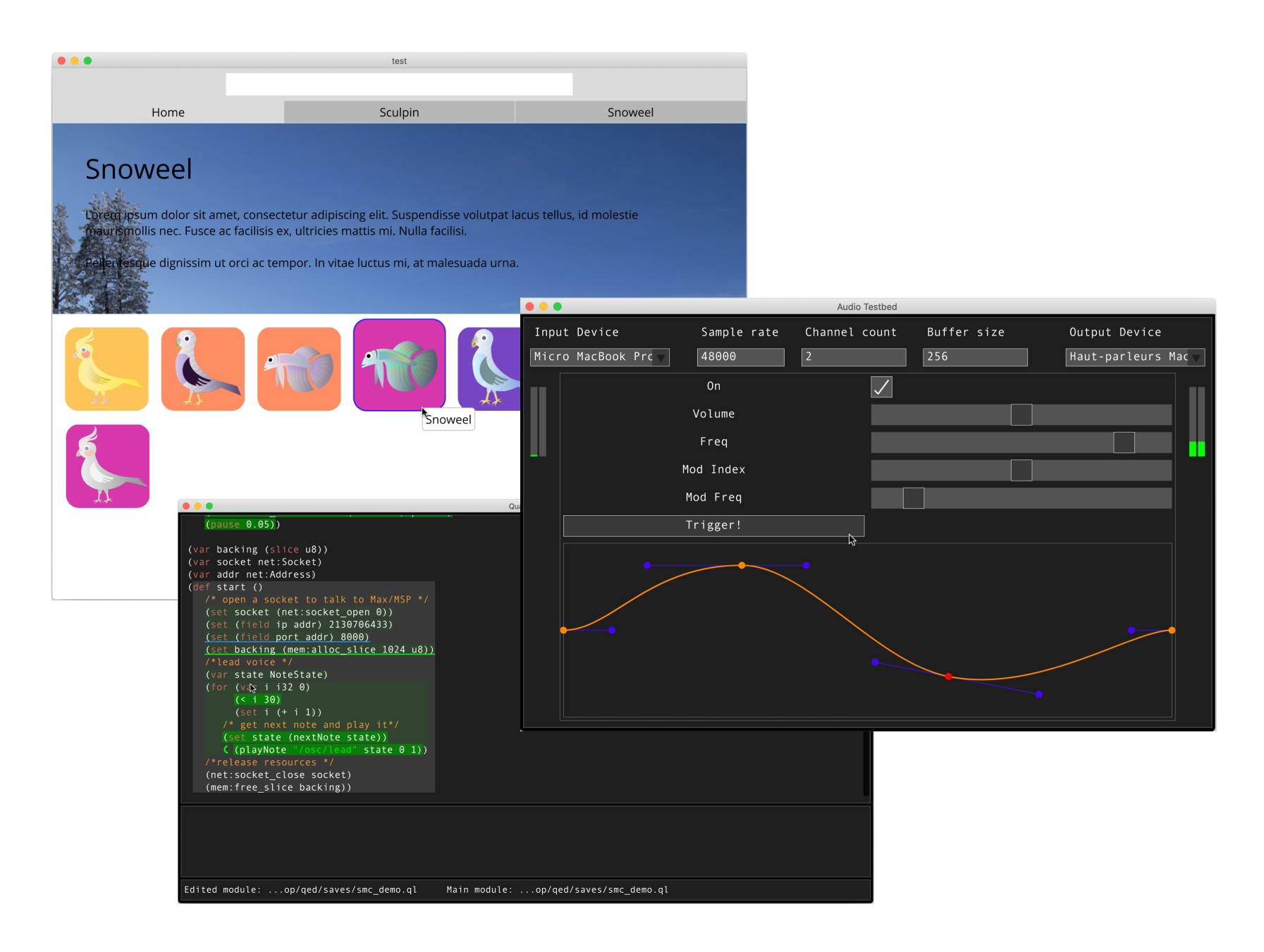
In this post, I’ll explain another set of techniques that better leverage the GPU and avoid curve subdivision and general polygon triangulation altogether. I’ve used this new renderer for some time now, for example to draw the UI of Quadrant and my two Handmade Network jam projects, Audio Testbed and Orca (Figure 1). There are still some things to iron out, but I figured I could do a write-up on the techniques I used, both to remind my future self of how it all works, and as an update to the previous series.

I was inspired by reading this post by Evan Wallace. They use a triangle fan algorithm described in (Haines 1994), though they implement it with a color blending trick instead of relying on the stencil buffer. They compute quadratics Bézier curves coverages using an implicitization method found in (Loop and Blinn 2005).

I expanded on these ideas to handle multiple overlapping shapes, as well as cubic Bézier outlines. The implementation is also different, as it relies on compute shaders, instead of additive blending and color buffers, so it doesn’t impose a low limit on the number of vertices per polygon. I also added a tiling pass, which considerably improves performance, especially when drawing a lot of small shapes such as glyphs.

Point in Polygon

Let’s first consider the problem of filling an arbitrary polygon. For each pixel \(P\), we can use the even-odd rule to determine if the pixel lies inside or outside the polygon:

We consider a ray from \(P\) to infinity and count the number of edges it crosses. If the ray crosses an odd number of edges, \(P\) lies inside the polygon. If the count is even, \(P\) lies outside the polygon.

Instead of directly checking each edge for intersection, we use the following method, described in (Haines 1994):

We choose an arbitrary point \(T\) and build a triangle fan from \(T\) to each edge of the polygon. We count the number of triangles that contain the point \(P\). If this count is odd, \(P\) lies inside the polygon. Otherwise it lies outside the polygon.

This method is equivalent to applying the even-odd rule on a ray emanating from \(P\) and in the direction of vector \(\overrightarrow{TP}\) (see Figure 3). This reduces our problem to a collection of point in triangle tests, which can be done by computing the barycentric coordinates of \(P\) with respect to each triangle.

We can choose any point as the apex of our triangle fan, but to avoid long thin triangles, it is best to chose one that is not too far away from the polygon’s centroid. For simplicity reasons, I just choose the first point of the polygon.

Note the test also works for polyline paths that describe multiple polygons, or polygon with holes. The test could also be extended to use the non-zero winding rule instead of the even-odd rule, by taking into account the orientation of the edges.

Curved Paths

We now consider a set of closed outlines that may contain curved edges described by Bézier curves. This can be decomposed as filling a polygonal path replacing each curve by a line segment, and then adding or subtracting the areas between the actual outline and that polygonal path (Figure 4).

This gives us the following method to test if a pixel \(P\) is inside or outside the outline:

• We first compute the crossing number of \(P\) with respect to the polygonal outline, as described above.
• For each curve, if \(P\) is between the curve and the segment joining its end points, we increment the crossing number.
• At the end, we apply the even-odd rule to our updated crossing number to determine if the point lies inside or outside the outline.

This effectively adds the areas that extend outside the polygonal outline, and carves out the ones that overlap with it.

We now need a way to determine if a pixel lies between a Bézier curve and the line segment joining its end points. We use the implicitization method described in (Loop and Blinn 2005). This method maps quadratic or cubic Bézier curves to one of a few canonical curves that can be described by a simple implicit curve equation. The coordinates of each control point in the canonical space are computed and affected as vertex attributes to this control point, similar to texture coordinates. The coordinates of an arbitrary point \(P\) in canonical space can be computed by interpolating the canonical space coordinates of control points. The implicit curve equation can then be evaluated to determine on which side of the curve the point lies.

For quadratic Bézier curves, the canonical space coordinates \((u, v)\) of control points \(b_0\), \(b_1\), \(b_2\) are respectively \((0, 0)\), \((\frac{1}{2}, 0)\) and \((1, 1)\), and a point lies between the curve and the segment joining its end points\((b_0, b_1)\) if \(u^2-v \leq 0\).

Cubic Bézier curves are a little more involved. We first need to classify the curve as the image of one of three canonical curves. Each canonical curve yields a different formula for computing canonical space coordinates \((k, l, m)\) of control points. A point lies between the curve and the segment joining its end points if \(k^3-lm \leq 0\). The classification of the curve and computation of canonical space coordinates to affect to control points can be done in constant time and involves a few matrix operations.

We can actually handle both quadratic and cubic curves, as well as plain triangles, with an implicit equation of the form \(k^3-lm \leq 0\):

• For plain triangles, we can set \(k\), \(l\) and \(m\) to 1, which means points inside the triangle always pass the test.
• For quadratic bézier curves, we can use \(k=u\), \(l=v\), \(m=u\). The test is then equivalent to \(u(u^2-v) \leq 0\), but since we know that in the quadratic case \(u\) is either \(0\), \(\frac{1}{2}\) or \(1\), this is equivalent to testing \(u^2-v \leq 0\).

Renderer Pipeline

Now we can put things together and outline the operation of our renderer. We start with a path that may contain multiple closed sub-paths. Each path section contains from 2 to 4 control points. A prepass is performed on the CPU side to prepare a vertex buffer to pass the GPU. Each vertex contains the following attributes:

• The vertex screen coordinates.
• The \((k, l, m)\) canonical curve space coordinates affected to the vertex.
• The color attribute of the vertex.

We also prepare an index buffer that indexes triangles inside the vertex buffer. The buffers are then processed by several compute shaders to render the filled outline onto an output texture.

Note that the vertex buffer is actually implemented as a structure of arrays: it consists of several buffers, one per vertex attributes. This avoids feeding unnecessary attributes to stages of our compute pipeline that don’t need them.

We now detail each stage of the pipeline.

On the CPU side

Let \(S\) be the starting point of the path. For each path edge \(E\) with control points \(p_0, ... p_n\), $ 2 n $:

• We push the triangle \((S, p_0, p_n)\) with the \((k, l, m)\) coordinates of vertices set to \((1, 1, 1)\).
• If the edge is a quadratic Bézier curve, we push the triangle \((p_0, p_1, p_2)\) with curve space coordinates respectively set to \((0, 0, 0)\), \((0.5, 0, 0.5)\) and \((1, 1, 1)\).
• If the edge is a cubic Bézier curve:
  • We categorize the curve and compute the \((k, l, m)\) coordinates of control points according to the curve type (this may split the curve at a double point and restart the computation for each part, but this can’t recurse further). We push the four vertices into the vertex buffer.
  • We use Jarvis’ march algorithm (Jarvis 1973) to compute the convex hull of the control points.
  • If the convex hull is a quad, we triangulate it along a diagonal. If it is a triangle, we split it in three triangles by adding edge from the inner control point to the other control points.
  • It might be necessary to flip the inside test in some of the triangles, so that the covered area is always the area between the curve and the segment joining \(p_0\) and \(p_1\). In order to do that, we modify our inside test by adding additional coordinate \(s\) in the test formula, yielding the test \(s\,(k_3-lm) \leq 0\). We can then set \(s\) to either \(1\) or \(-1\) depending on if we want to flip the inside and outside areas. We compute the inside test on the one or two inner control points that are part of the convex hull. If necessary, we flip the test in the triangles containing these points, so that they lie outside the covered area.

Once the vertex and index buffers are filled, the kick off our compute pipeline on the GPU side.

On the GPU side

The compute shader to fill outlines is rather simple. It runs for each pixel and determines if it is covered by the filled shape as follows:

• Initialize a coverage counter to 0.
• For each triangle:
  • compute the barycentric coordinates of the pixel. If one of them is outside \([0, 1]\), skip this triangle.
  • Otherwise, compute the \((k, l, m, s)\) values for the pixel by weighting the \((k,l,m, s)\) coordinates of the triangle’s vertices with the barycentric coordinates.
  • If \(s\,(k_3-lm) \leq 0\), increment the coverage counter.
• At the end, if the counter is odd, the pixel lies outside the outline and is discarded. If it’s even, it lies inside the outline and its color is written to the output texture.

Triangle Rasterization Caveats.

We glossed over an important detail regarding the point in triangle test. Points lying on a edge shared by two triangles must be covered by only one triangle, lest we would create visible seams inside our shape and lines outside it. Thus the computation of triangle coverage must include a tie-breaking rule when two triangles compete for the same edge. The implementation of such a rule is explained (along with many other aspect of triangle rasterization) in this post by Fabian Giesen. Essentially, top and left edges of triangles are counted as covered by the triangles, but other edges are not.

Supporting overlapping and transluscent shapes

Distinct overlapping shapes can be drawn using this method by adding a shape counter to the vertex attributes, and incrementing the shape counter each time the CPU prepass processes a new shape. In the compute shader, we can then distinguish batches of triangles belonging to the same shape:

• Initialize the current shape counter to the shape counter of the first triangle.
• Compute coverage as described above, until we encounter a triangle whose shape counter is greater than the current shape counter.
• Depending on the value of the coverage counter, discard or write the color to a temporary color variable. Reinitialize the coverage counter, update the shape counter, and start a new batch.
• At the end, write the temporary color variable to the output texture.

Instead of overwriting the temporary color variable, the color of each covering batch can be blended with the previous value, which allows rendering transparent overlapping shapes.

Anti-Aliasing

For anti-aliasing I just compute multiple samples per pixels by wrapping the algorithm described above in a loop, and blend them before writing to the output texture.

Texturing

I described solid color shapes, but the technique can also be used to draw textured shapes. We can affect texture coordinates to the control points of the path and path them along as vertex attributes. In the rendering shader, we can sample a color value from a texture and multiply it with the interpolated color attribute before blending the result into the temporary output color. This allows rendering both textured shapes (with a solid white color) and colored shapes (with a white texture), as well as tinted textured shapes (multiplying a texture with a solid color).

Stroking

To stroke polylines with caps and joins I use the same triangulation as described in my previous series.

Bézier curves can be stroked by generating and outline from two offset versions of the curve and filling that outline. Unfortunately, the offset curve of a cubic Bézier curve is not itself a cubic Bézier curve. However, we can approximate it with a cubic Bézier using the Tiller-Hanson algorithm (Tiller and Hanson 1984), and subdivide the curve until we reach a desired accuracy.

Tiled Renderer

It is undesirable to check every pixel against every triangle generated by our outlines. For this reason I added a tiling prepass to the renderer. The screen is divided into 16x16 pixels tiles. Pixels in a tile only check coverage against triangle whose axis-aligned bounding box intersects the tile.

We reserve a large buffer and divide it into sections called triangle buffer arrays, one per tile. Each element of a triangle buffer array points to a slot in the index buffer. That slot is the first of three consecutive slots indexing a triangle (See Figure 5). Each tile also has an atomic counter that holds the number of triangle indices contained in the triangle index buffer of that tile.

The tiling mechanism involves several compute shaders:

• A bounding box kernel is run for each triangle and computes its axis-aligned bounding box.
• A tiling kernel runs for each triangle. It computes the span of rows and columns of tiles intersected by the bounding box, by dividing the box corner coordinates by the tile size and flooring the result. It then runs a double loop through this set of tiles and appends the triangle to each tile’s triangle index buffer, by doing an atomic fetch and add on the tile counter and storing the triangle index at the position indicated by the old counter value.
• We then run a sorting kernel on each tile triangle index buffer, to make sure triangles belonging to the same shapes are contiguous. This is necessary even though triangle are initially sorted, because the tiling kernel might have interleaved triangles belonging to different shapes in the triangle index buffer.
• We then run the render kernel for each pixel:
  • We first get the tile index by dividing the pixel coordinates by the tile size
  • We get the tile’s counter and triangle index buffer. We run the coverage tests described above against all triangles referenced in the triangle index buffer, and write the color value of the pixel to the output texture.

Wrap-up

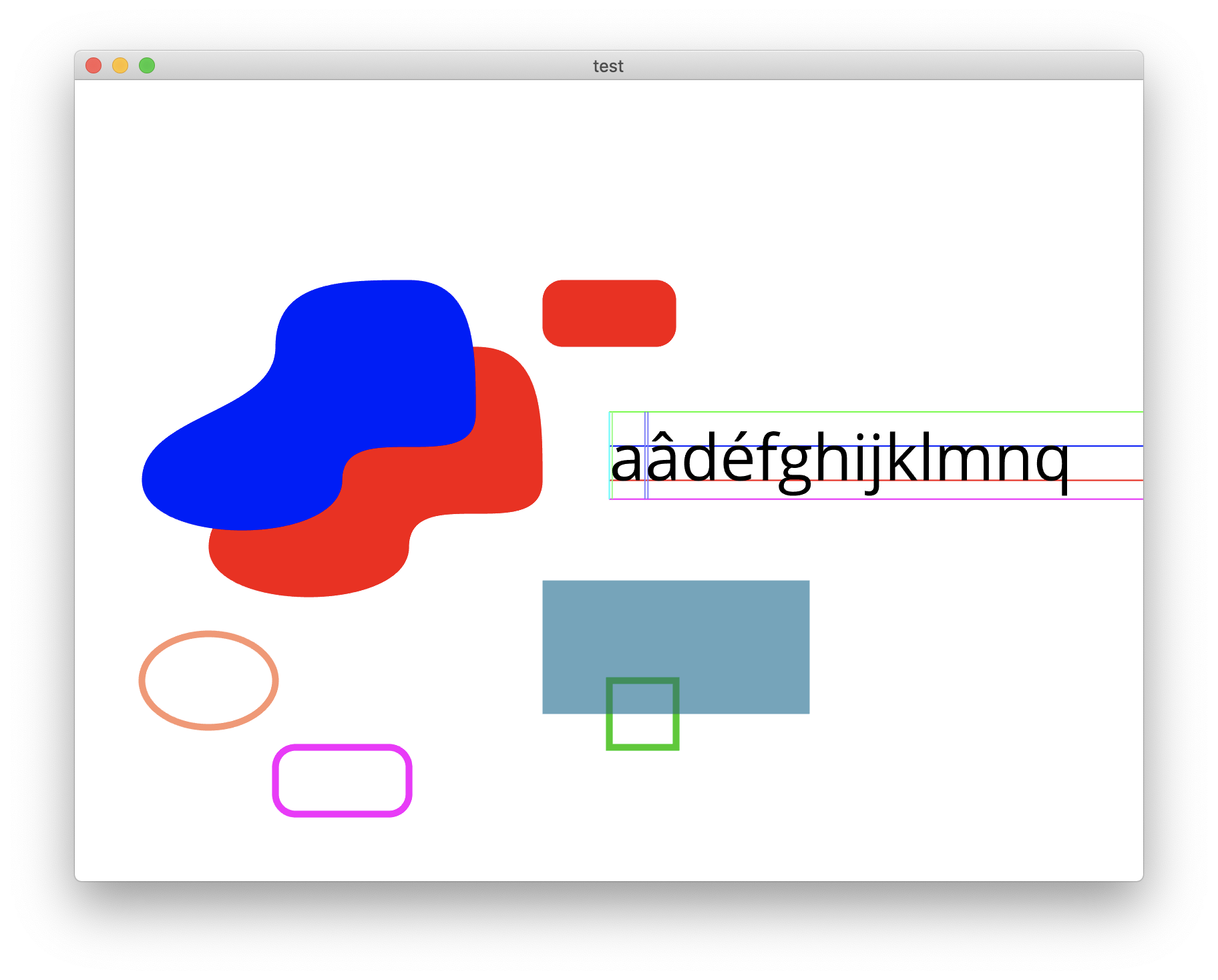
This is all for today! Here is a screenshot showcasing some anti-aliased stroked and filled paths, with overlapping and transluscent shapes:

Let’s recap the steps needed to fill a path using the techniques described in this post:

• You start with an outline containing curved edges.
• You generate a triangle fan for the polygonal outline, ignoring curves
• You generate triangles for the curves, and set the \((k,l, m, s)\) coordinates of each vertex to the values computed using the Loop-Blinn implicitization method.
• On the GPU, you apply the tiling prepass to bin triangles into screen tiles.
• The rendering kernel then runs for each sample and computes coverage against each triangle in the tile’s triangle buffer. Colors of overlapping shapes are blended into a temporary color variable. Finally, the resulting color is written to the output texture.

The advantages of this method are:

• It avoids Bézier curve subdivision with its accuracy/performance tradeoff.
• It avoids \(O(n\,\text{log}\,n)\) general polygon triangulation.
• It generates a lot less triangles to pass to the GPU.

This said, there are disadvantages:

• It is in my opinion harder to grok than the simple subdivision and triangulation method.
• It is prone to numerical accuracy issues, some of which I still have to iron out.

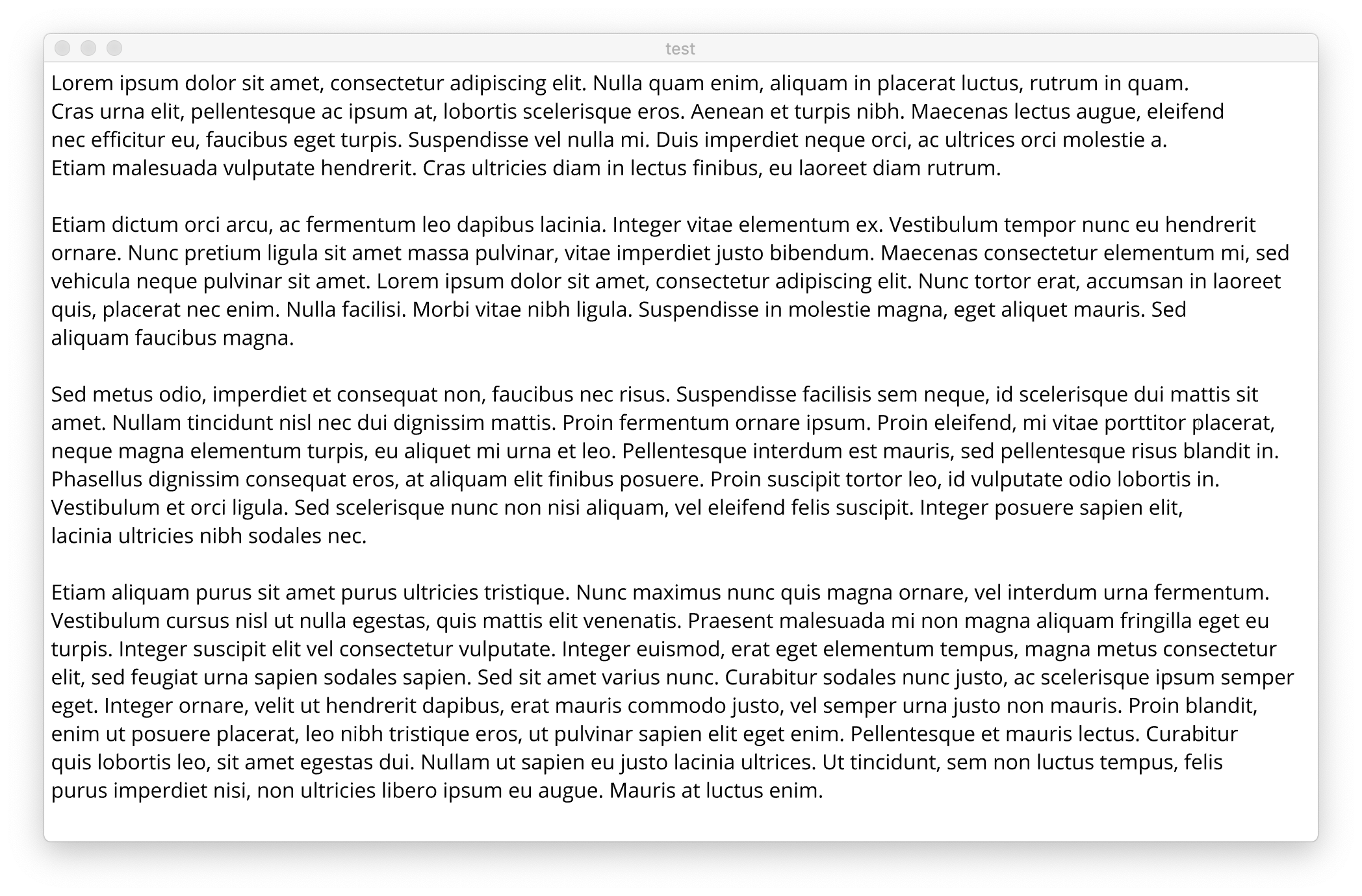
I haven’t done serious optimization work yet (it already worked quite alright for my UI needs!), but a very cursory test seems to indicate that rendering a lorem ipsum text (Figure 7) containing 2626 glyphs for a total of 66765 triangles takes around 14ms, divided between approximately 3.5 ms on the CPU and 10.5 ms on the GPU, on my 2019 MacBook Pro. That is around 5\(\mu\)s per glyph.

Overall it’s been pretty good for my UI needs, as I can simply redraw the UI each frame at 60fps without having to keep track of dirty rectangles or caching text, as was needed with my previous renderer.

I suspect there is yet more parallelism to be extracted from the tiling and rendering passes, and that some perparation work that we currently do on the CPU could be uploaded to the GPU. I’ll update this post when I finally get to do some serious benchmarking!

References